The standard-star fields of the Southern Standard Stars For The u´, g´, r´, i´, z´ System (hereafter SSS) were observed in both 2013 and 2014. The Sloan Digital Sky Survey Stripe82 regions were observed in 2013. The magnitude differences Δm between our measurement maper and the standard star catalog mss are fitted into two terms, a and b, for intercept and slope as a function of the airmass (Z), respectively:
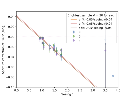
\begin{equation} m_{ss} = m_{aper} + a + b * Z \ , \tag{1} \end{equation}For maper, we adopt the MAG_APER values from the SExtractor running at radii 14.8″ (following Smith et al. 2003; Sheen et al. 2012) after the aperture correction for various seeing (see Figure 1).

We set the instrumental zero point as 25 tentatively. We use the weighted linear regression model class WLS contained in the Python library statsmodel for fitting. The quadratic sum of the errors of mss and maper are weighted. The sources having either:
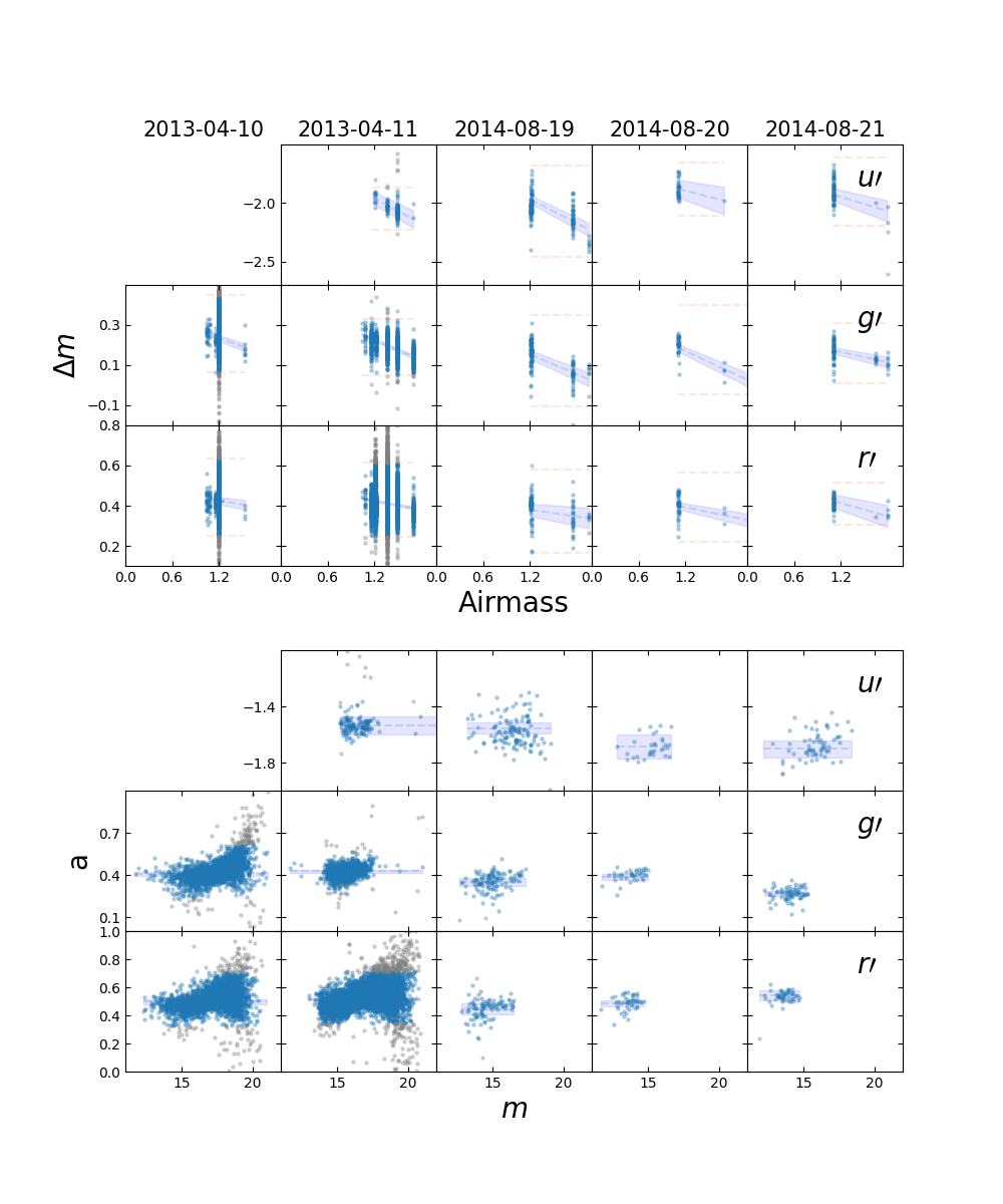
Figure 2 shows the result. The columns are ordered by observing dates and the rows are ordered by filters and fitted parameters. Upper panels for each filter are for b in Equation 2 and lower ones are for a. In the upper panels, the slope as a function of the airmass b is drawn as a dashed blue line and the shaded region represents the uncertainty. The 3-σ limits are shown as pink dashed lines. Lower panels show fitting for \(a, \Delta m - b * Z\), as a function of the magnitudes of the standard stars m. Fitting results for a the uncertainty is drawn as a dashed blue line and the blue shaded region, respectively. The resulting values of a and b for each filter and date are listed in Table 1 with the number of point sources.

| Date | Filter | a | b | # of sources |
|---|---|---|---|---|
| 2013-04-10 | g´ | 0.408±0.015 | -0.143±0.012 | 2433 |
| r´ | 0.498±0.018 | -0.061±0.015 | 3804 | |
| 2013-04-11 | u´ | -1.534±0.063 | -0.355±0.044 | 134 |
| g´ | 0.426±0.009 | -0.166±0.006 | 1281 | |
| r´ | 0.513±0.005 | -0.073±0.004 | 9239 | |
| 2014-08-19 | u´ | -1.555±0.041 | -0.342±0.028 | 132 |
| g´ | 0.350±0.026 | -0.163±0.018 | 120 | |
| r´ | 0.445±0.038 | -0.054±0.026 | 97 | |
| 2014-08-20 | u´ | -1.686±0.083 | -0.172±0.069 | 32 |
| g´ | 0.385±0.024 | -0.179±0.017 | 40 | |
| r´ | 0.488±0.022 | -0.080±0.016 | 48 | |
| 2014-08-21 | u´ | -1.702±0.062 | -0.203±0.050 | 65 |
| g´ | 0.268±0.021 | -0.085±0.015 | 73 | |
| r´ | 0.544±0.035 | -0.109±0.030 | 49 |
We calibrate single-exposure images first because we can not directly calibrate the deep combined images which are stacks of the multiple single-exposure images. The best single images for each cluster and band was chosen assessing the airmass and the seeing values. The exposure times and dates of the best single images are presented in Table 1 of Kim et al. (in prep). We ran SExtractor version 2.25.0 on 60--61 tiles in the mosaic separately plugging the point-spread function (PSF) model for each tile. We used PSFEx to model the PSFs. We use MAG_BEST for magnitudes of the single and combined images. The MAG_BEST is more robust than MAG_AUTO when sources are crowded. We calibrate magnitudes of sources in single images by using a and b values obtained from the previous chapter.
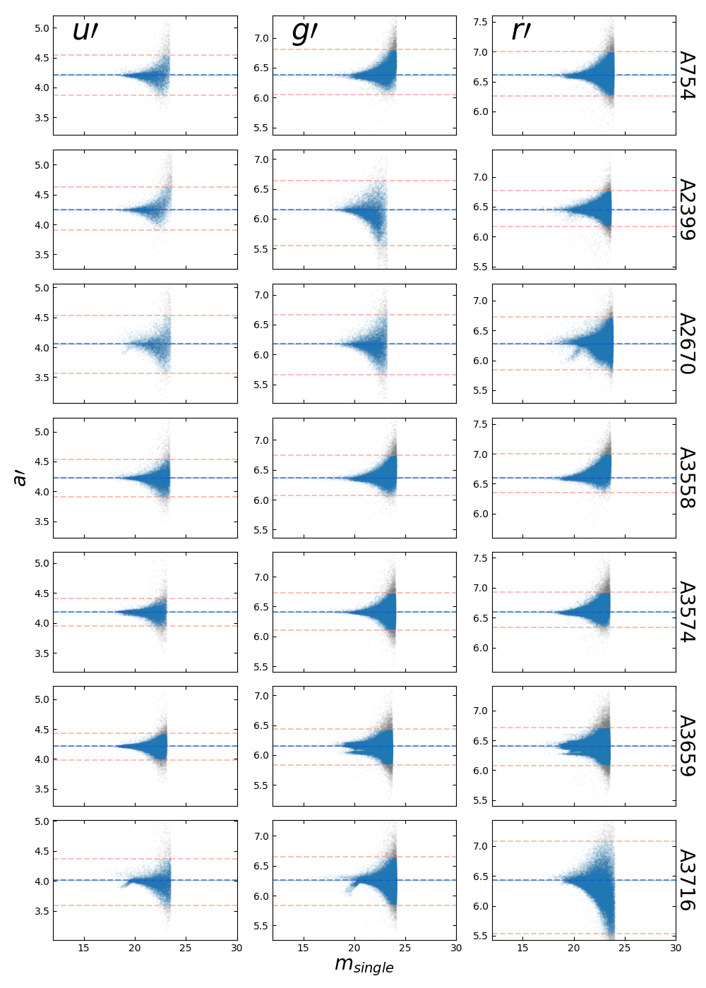
We ran SExtractor on the deep combined images in a similar way to the single images. We calibrate then the magnitudes of the SExtractor catalogs of the combined images by fitting zero points of each image. To do that, we linearly fit the magnitude differences between the matched sources between the single and the combined images after setting arbitrary zero points of the combined images as 25. For the fitting, we used the WLS with the 3-σ clipping same as the standard-star calibration process.
\begin{equation} m_{single} - m_{combined, ZP=25} \ (\Delta m\prime) = a\prime \ . \tag{3} \end{equation}Sources having either:

For more information please refer to Kim et al. (in prep), or
Send an email to duhokim81@gmail.com